MATLAB / Octave Tutorial----Chapter 3-----Visualising the data(Part 3)

Chapter 3: Visualising the data

Part 3

Welcome to the third and the final part of this chapter. In this part, you'll come to learn how to plot complex(not in the mathematical sense!) functions. But before that, I shall show you some more tools about visualising the data.

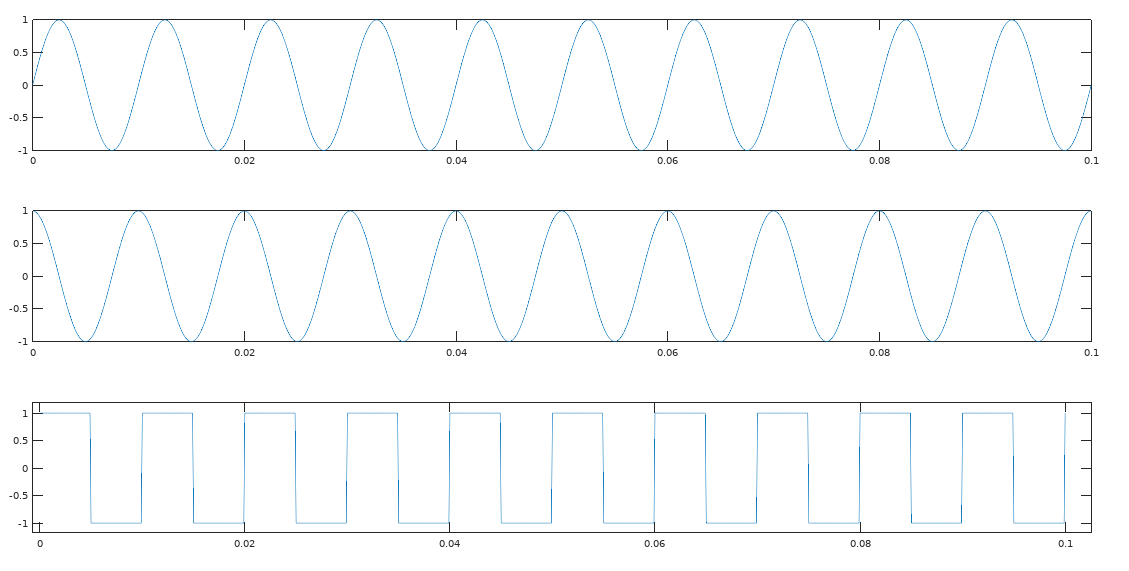
The first one is, subplot. This method is used for plotting different graphs on a single figure/window. The syntax for subplot is: subplot(a,b,c). Here, a is the number of rows in which the figure has to be divided into, b is the number of columns and c denotes the subdivision where we want to plot the graph. For example, subplot(2,1,1) means: Divide the graph into two rows and one column and plot the graph in the first subdivision.

Fig 1: Demonstration of subplots

We shall type the following on the command window and see the output.

The output is shown below:

Let's see a few more subplot examples:

You can try various other variations of subplots. However, always remember, total number of subdivisions will be equal to number of rows multiplied by number of columns.

You can also generate a new figure/plotting window using the figure command like so:

Fig 2: Demonstration of figure command

Now, let us learn how to plot intricate mathematical expressions using MATLAB/Octave.

Let's consider a function like this: y = 2x + 3. In this function, x is the independent variable and y is dependent on x. In order to plot this  function we need to assign some values to x and in that course, some values of y will be generated. It might nit be practical to manually assign tens or hundreds of values to x. So, MATLAB provides a simple means to do that.

We can assign values to x like this: x = 0 : 10

This means, the values of x range from 0 to 10 at intervals of 1. We can also assign x like this:

x = 0 : 0.1 : 10. This means that, x has values ranging from 0 to 10 at intervals of 0.1. In the first case, there will be only 11(0 to 10) values of x, whereas in the second case there will be 101 values of x(0 to 100). Let's implement this on the compiler:

Now, let us see what values of y we get with these values of x:

Now, I shall write this MATLAB script to print the graphs of various fuctions.

Now, let us see what type of graphs are generated:

Here we come to the end of this tutorial lesson. I hope, this lesson will help you realise mathematical functions with MATLAB. For your practice, I give you some assignment questions. Please practice it and upload it to Request folder in GitHub from the link given in comment section. Also, you can find the MATLAB script in the Tutorial folder. Happy Learning!!!